Making Noise
Original presentation was made by Ken Perlin. I've found it in the web archive and want to make it more accessible. It covers the history of creating shader concept, and should be the bible of every developer who generates textures.
Based on a talk presented at GDCHardCore on Dec 9, 1999
Making Noise by Ken Perlin
Slide 1 | Structure of this talk
In this talk I'm going to take you on a tour, first of how and why I developed noise, then of some examples of how it's been used, then how it's constructed. Finally, I'll talk about my current work in building it right into hardware, at the gate array level, and I'll ed with some comments about future work.
Slide 2 | What's noise?
Noise is a texturing primitive you can use to create a very wide variety of natural looking textures. Combining noise into various mathematical expressions produces procedural texture.
Unlike traditional texture mapping, procedural texture doesn't require a source texture image. As a result, the bandwidth requirements for transmitting or storing procedural textures are essentially zero.
Also, procedural texture can be applied directly onto a three dimensional object. This avoids the "mapping problem" of traditional texture mapping. Instead of trying to figure out how to wrap a two dimensional texture image around a complex object, you can just dip the object into a soup of procedural texture material. Essentially, the virtual object is carved out of a virtual solid material defined by the procedural texture. For this reason, procedural textures are sometimes called solid texture.
Slide 3 | History

I first started to think seriously about procedural textures when I was working on TRON at MAGI in Elmsford, NY, in 1981. TRON was the first movie with a large amount of solid shaded computer graphics. This made it revolutionary. On the other hand, the look designed for it by its creator Steven Lisberger was based around the known limitations of the technology.
Lisberger had gotten the idea for TRON after seeing the MAGI demo reel in 1978. He then approached the Walt Disney Company with his concept. Disney's Feature Film division was then under the visionary guidance of Tom Wilhite, who arranged for contributions from the various computer graphics companies of the day, including III, MAGI, and Digital Effects.
Working on TRON was a blast, but on some level I was frustrated by the fact that everything looked machine-like. In fact, that became the "look" associated with MAGI in the wake of TRON. So I got to work trying to help us break out of the "machine-look ghetto."
Slide 4 | History
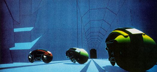
One of the factors that influenced me was the fact that MAGI SynthaVision did not use polygons. Rather, everything was built from boolean combinations of mathematical primitives, such as ellipsoids, cylinders, truncated cones. As you can see in the illustration on the left, the lightcycles are created by adding and subtracting simple solid mathematical shapes.
This encouraged me to think of texturing in terms not of surfaces, but of volumes. First I developed what are now called "projection textures," which were also independently developed by a quite a few folks. Unfortunately (or fortunately, depending on how you look at it) our Perkin-Elmer and Gould SEL computers, while extremely fast for the time, had very little RAM, so we couldn't fit detailed texture images into memory. I started to look for other approaches.
Slide 5 | Controlled random primitive
Lets implement the Perlin noise!
The first thing I did in 1983 was to create a primitive space-filling signal that would give an impression of randomness. It needed to have variation that looked random, and yet it needed to be controllable, so it could be used to design various looks. I set about designing a primitive that would be "random" but with all its visual features roughly the same size (no high or low spatial frequencies).
I ended up developing a simple pseudo-random "noise" function that fills all of three dimensional space. A slice out of this stuff is pictured to the left. In order to make it controllable, the important thing is that all the apparently random variations be the same size and roughly isotropic. Ideally, you want to be able to do arbitrary translations and rotations without changing its appearance too much. You can find my original 1983 code for the first version here.
My goal was to be able to use this function in functional expressions to make natural looking textures. I gave it a range of –1 to +1 (like sine and cosine) so that is would have a dc component of zero. This would make it easy to use noise to perturb things, and just "fuzz out" to zero when scaled to be small.
// Adapted C code from http://mrl.nyu.edu/~perlin/doc/oscar.html

var B = 0x100,
  BM = 0xFF,

  N = 0x1000,
  NP = 12, /* 2^N */

  NM = 0xFFF,

  p = [], g2 = []

for(var i = 0; i < B+B+2; i++) {
  p[ i ] = 0;
  g2[ i ] = [0, 0];
}


var lerp = (t, a, b) => ( a + t * (b - a) );
var at2 = (rx,ry, q) => ( rx * q[0] + ry * q[1] );
var s_curve = (t) => ( t * t * (3. - 2. * t) );

var normalize2 = (v)=>{
  var s = sqrt(v[0] * v[0] + v[1] * v[1]);
  v[0] = v[0] / s;
  v[1] = v[1] / s;
}

var noise2 = function(x, y){

  var vec = [x,y];
  var bx0, bx1, by0, by1, b00, b10, b01, b11;
  var rx0, rx1, ry0, ry1, q, sx, sy, a, b, t, u, v;
  var i, j;

  //setup(0, bx0,bx1, rx0,rx1);
  //#define setup(i,b0,b1,r0,r1)
  t = vec[0] + N;
  bx0 = (t|0) & BM;
  bx1 = (bx0+1) & BM;
  rx0 = t - (t|0);
  rx1 = rx0 - 1.;

  //setup(1, by0,by1, ry0,ry1);
  t = vec[1] + N;
  by0 = (t|0) & BM;
  by1 = (by0+1) & BM;
  ry0 = t - (t|0);
  ry1 = ry0 - 1.;

  i = p[ bx0 ];
  j = p[ bx1 ];

  b00 = p[ i + by0 ];
  b10 = p[ j + by0 ];
  b01 = p[ i + by1 ];
  b11 = p[ j + by1 ];

  sx = s_curve(rx0);
  sy = s_curve(ry0);

  q = g2[ b00 ] ; u = at2(rx0,ry0,q);
  q = g2[ b10 ] ; v = at2(rx1,ry0,q);
  a = lerp(sx, u, v);

  q = g2[ b01 ] ; u = at2(rx0,ry1,q);
  q = g2[ b11 ] ; v = at2(rx1,ry1,q);
  b = lerp(sx, u, v);

  return lerp(sy, a, b);
}

var rnd = ()=> (-(2<<30)-1) *Math.random() |0

var init = () => {
  var i, j, k;

  for (i = 0 ; i < B ; i++) {
    p[i] = i;


    for (j = 0 ; j < 2 ; j++)
      g2[i][j] = ((rnd() % (B + B)) - B) / B;

    normalize2(g2[i]);

  }

  while (--i) {
    k = p[i];
    p[i] = p[j = rnd() % B];
    p[j] = k;
  }

  for (i = 0 ; i < B + 2 ; i++) {
    p[B + i] = p[i];
    for (j = 0 ; j < 2 ; j++)
      g2[B + i][j] = g2[i][j];

  }
};

init();
rect(0,0,w,h,0x000000);

update = function(dt, t){
  fillCircle(center.x, center.y, 120, function(x,y){
    var scale = 20+sin(t/4)*5;
    var noise = (noise2((x-w/2+sin(t/3)*8+t)/w*scale,(y-h/2 +cos(t/3)*8)/h*scale)/2+ 0.5) *0xFF |0;
    return noise + (noise << 8) + (noise << 16);
  } );
}Slide 6 | Think of it as seasoning
Noise itself doesn't do much except make a simple pattern. But it provides seasoning to help you make things irregular enough so that you can make them look more interesting.
The fact that noise doesn't repeat makes it useful the way a paint brush is useful when painting. You use a particular paint brush because the bristles have a particular statistical quality — because of the size and spacing and stiffness of the bristles. You don't know, or want to know, about the arrangement of each particular bristle. In effect, oil painters use a controlled random process (centuries before John Cage made such a big deal about it).
Noise allowed me to do that with mathematical expressions to make textures.
Slide 7 | Rapid adoption
In late 1983 I wrote a language to allow me to execute arbitrary shading and texturing programs. For each pixel of an image, the language took in surface position and normal as well as material id, ran a shading, lighting and texturing program, and output color. As far as I've been able to determine, this was the first shader language in existence (as my grandmother would have said, who knew?).
I treated normal perturbation, local variations in specularity, nonisotropic reflection models, shading, lighting, etc. as just different forms of procedural texture — I didn't see any reason to make a big distinction between them. I presented this work first at a course in SIGGRAPH 84, and then as a paper in SIGGRAPH 85. Because the techniques were so simple, they quickly got adopted throughout the industry. By around 1988 noise-based shaders where de rigeur in commercial software.
I didn't patent. As my grandmother would have said...
Slide 8 | 1989: Hypertexture
Meanwhile, I joined the faculty at NYU and did all sorts of research. One of the questions I was asking in 1988 and 1989 was whether you could use procedural textures to unify rendering and shape modeling. I started to define volume-filling procedural textures and render them by marching rays through the volumes, accumulating density along the way and using the density gradient to do lighting.
I worked with a student of mine, Eric Hoffert, to produce a SIGGRAPH paper in 1989. The technique is called hypertexture, officially because it is texture in a higher dimension, but actually because the word sounds like "hypertexture" and for some reason I thought this was funny. I offer no redeeming excuse.
The image on the left is of a procedurally generated rock archway. Like all hypertextures, it's really a density cloud that's been "sharpened" to look like a solid object. I defined this hypertexture first by defining a space-filling function that has a smooth isosurface contour in the shape of an archway. Then I added to this function a fractal sum of noise functions: at each iteration of the sum I doubled the frequency and halved the amplitude. Finally, I applied a high gain to the density function, so that the transition from zero to one would be rapid (about two ray samples thick). When you march rays through this function, you get the image on the left.
Slide 9 | Hypertexture
I tried to make as many different materials as possible. On the left is one of a series of experiments in simulating woven fabric. To make this, I first defined a flat slab, in which density is one when y=0, and then drops off to zero when y wanders off its zero plane. More formally: f(x,y,z) = {if |y| > 1 then 0 else 1 - |y|}.
I made the plane ripple up and down by replacing y with y + sin(x)*sin(z) before evaluating the slab function. Then I cut the slab into fibers by multiplying the slab function by cos(x). This gave me the warp threads of a woven material. Finally, I rotated the whole thing by 90o to get the weft threads. When you add the warp and the weft together, you get something like the material on the left.
To make the fiber more coarse (ie: wooley) or conversely more fine, I modulated the bias and gain of the resulting function. To make the surface undulate, I added low frequency noise to y before evaluating anything. To give a nice irregular quality to the cloth, I added high frequency noise into the function.
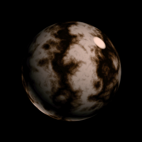
Slide 10 | Hypertexture
I also made a tribble, as shown on the left, as well as other experiments in furrier synthesis. Here I shaped the density cloud into long fibers, by defining a high frequency spot function (via noise) onto an inner surface, and then, from any point P in the volume, projecting down onto this surface, and using the density on the surface to define the density at P. This tends to make long fibrous shapes, since it results in equal densities all along the line above any given point on the inner surface.
I made the hairs curl by adding low frequency noise into the domain of the density function. This was the first example in computer graphics of long and curly fur. Around the same time Jim Kajiya made some really cool fur models, although his techniques produced only short and straight fur. Jim had the good sense to use earthly plushy toys for his shape models, instead of alien ones. The earthly ones are more easily recognized by the academy...
Slide 11 | Hypertexture
It has always seemed to me that there would be advantages in having optical materials with continually varying density, within which light travels in curved paths. The image on the left is a hypertexture experiment in continuous refraction. The object is transparent, and every point on its interior has a different index of refraction. I implemented a volumetric version of Snell's law, to trace the curved paths made by light as it traveled through the object's interior.
The background is not really an out-of-focus scene; it's just low frequency noise added to a color grad. This is a situation in which noise is really convenient - to give that look of "there's something in background, and I don't know what it is, but it looks reasonable and it sure is out of focus."
Slide 12 | Meanwhile, back at the Ranch
Meanwhile, back at the Ranch (if you're reading this you presumably know which ranch I'm talking about) the use of noise spread like wildfire. All the James Cameron, Schwartzenegger, Star Trek, Batman, etc. movies started relying on it.
Noise benefits from Moore's law: as computer CPU time becomes cheaper, production companies increasingly have turned away from physical models, and toward computer graphics. Noise is one of the main techniques production companies use to fool audiences into thinking that computer graphic models have the subtle irregularities of real objects.
Disney put it into their CAPS system - you can see it in the mists and layered atmosphere in high end animated features like The Lion King.
In fact, after around 1990 or so, every Hollywood effects film has used it, since they all make use of software shaders, and software shaders depend heavily on noise. Which is why I have finally gotten around to giving an up-to-date talk on how it works.
Slide 13 | How does it work?
The implementation of the noise function itself turns out not to be that complex. I will show how it is constructed, and various ways it is used in shader programs to get different kinds of procedural textures. There will be pictures and animations.
Finally I'll talk about a real-time implementation, which I designed so that it could be used most effectively in game hardware and other platforms that support noise-intensive imagery at many frames per second.
Slide 14 | Band limited repeatable random function
Noise appears random, but isn't really. If it were really random, then you'd get a different result every time you call it. Instead, it's pseudo-random — it gives the appearance of randomness.
Noise is a mapping from Rn to R — you input an n-dimensional point with real coordinates, and it returns a real value. Currently the most common uses are for n=1, n=2, and n=3. The first is used for animation, the second for cheap texture hacks, and the third for less-cheap texture hacks. Noise over R4 is also very useful for time-varying solid textures, as I'll show later.
Noise is band-limited — almost all of its energy (when looked at as a signal) is concentrated in a small part of the frequency spectrum. High frequencies (visually small details) and low frequencies (large shapes) contribute very little energy. Its appearance is similar to what you'd get if you took a big block of random values and blurred it (ie: convolved with a gaussian kernel). Although that would be quite expensive to compute.
To make noise run fast, I implement it as a pseudo-random spline on a regular grid. Now we'll examine this fast implementation in some detail.
Slide 15 | Algorithm
The outline of my algorithm to create noise is very simple. Given an input point P, look at each of the surrounding grid points. In two dimensions there will be four surrounding grid points; in three dimensions there will be eight. In n dimensions, a point will have 2n surrounding grid points.
For each surrounding grid point Q, choose a pseudo-random gradient vector G. It is very important that for any particular grid point you always choose the same gradient vector.
Compute the inner product G . (P-Q). This will give the value at P of the linear function with gradient G which is zero at grid point Q.
Now you have 2n of these values. Interpolate between them down to your point, using an S-shaped cross-fade curve (eg: 3t2–2t3) to weight the interpolant in each dimension. This step will require computing n S curves, followed by 2n–1 linear interpolations.
Click on item 3 to the left to follow these steps one by one.
Slide 16 | The 8 neighbors in three dimensions
In three dimensions, there are eight surrounding grid points. To combine their respective influences will require a trilinear interpolation (linear interpolation in each of three dimensions).
In practice this means that once we've computed the 3t2–2t3 cross-fade function in each of x,y and z, respectively, then we'll need to do seven linear interpolations to get the final result. Each linear interpolation a+t(b–a) requires one multiply.
In the diagram to the left, x,y,z are in the right,up and forward directions, respectively. The six white dots are the results of the first six interpolations: four in x, followed by two in y. Finally, a seventh interpolation in z gives the final result.
Slide 17 | Computing the pseudo-random gradient
Computing the gradient must be very fast, since we must this a number of times per evaluation of the noise function. It is also very important that there be no visible correlations between successive gradient values in any neighborhood. Otherwise, telltale correlation patterns will be visible. In particular, we need to pick our gradients in such a way that there will be no visible correlation between the gradient at integer grid point (i,j,k) and its neighbors at, say, (i+1,j,k), (i,j+1,k) or (i,j,k+1).
Fortunately, it is ok for the noise function to repeat, as long as it repeats only after long distance. After a distance of a few hundred units, it doesn't matter if the same pattern appears again. The noise function has no large-scale features, so by the time an observer is zoomed out far enough to see a repeat pattern, the whole noise texture is too small to see anyway.
Keeping this in mind, the method I came up with in 1983 for noise over R3 was to make a solid tiling block 2563 in size. I did this by precomputing a permutation table P with 256 entries, which scrambles up the order of the numbers from 0 through 255. I also precomputed a table of gradients G with 256 entries. Then I applied the modular arithmetic trick shown on the left. By alternating between permuting and index addition, I was able to create a pattern of apparently random gradients for any input (0,0,0) ≤ (i,j,k) ≤ (255,255,255).
Actually, you don't really need to call a mod function; since 256 is a power of two, I just did the addition and masked off all but the lowest 8 bits, so the actual computational cost is really more like what you now see on the left.
To precompute the table of gradients G, I did a Monte Carlo simulation, as follows:
The problem was to compute 256 gradient vectors uniformly around the surface of a sphere. I knew that I could compute points uniformly within a cubic volume, by picking uniformly random values of x,y, and z via a rand() function.
In order to make a uniformly random distribution of points on the surface of a sphere, you really just need to make a uniformly random distribution of points within a spherical volume. Then you can normalize them (ie: resize them all to unit length).
So my Monte Carlo simulation worked as follows: I generated uniformally random points within the cube which surrounds the unit sphere. I threw out all the points that lie outside the unit sphere and kept all the points that lie inside the unit sphere. These are the points for which x2+y2+z2 < 1.
I stopped this process only when I had filled up a table of 256 entries. I then normalized all the entries in the table, and I was done.
Slide 18 | Use in expressions to get texture
Noe I'll go through a series of examples to show how you can use noise within simple expressions to make cool and natural looking textures. By varying the terms in the expressions you can get a wide variety of effects, including rock, mountains, wood, fire, marble, smoke, clouds, water, stucco (oh, can you get stucco…), lava, skin, oil films, and many others.
Slide 19 | Use in expressions to get texture
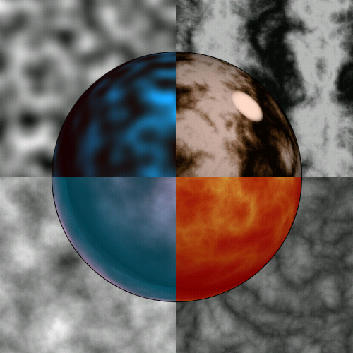
The image on the left is a sphere sticking out of a flat plain. For each of the four textures shown, I computed an expression using noise, and evaluated it on the plane so you could see what the texture looks like. Then I took the same texture, added some color table and lighting stuff, and evaluated it on the surface of the sphere.
It is clear from this composite image that 3D lighting and color remapping add a lot, and are very effective in completing the look of noise-based textures.
There is a natural progression in the examples on the left, and in the next few slides we'll be going through them one at a time. It's best to read the image starting at the top-left (just noise) and going counter-clockwise, ending at the top right marble image. In each successive image the expression using noise is made a little fancier, and the resulting look changes.
Slide 20 | noise
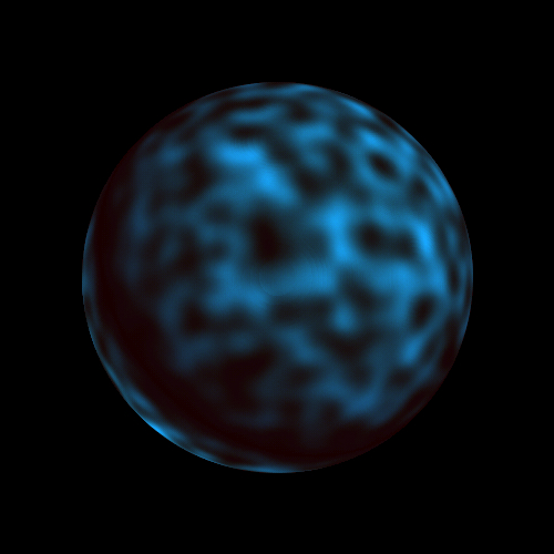
Just applying noise itself to modulate surface color has some utility, but only in limited situations. It's great for making objects appear subtly dirty or worn by adding color variations over a surface. You can also use it to vary a specular power, to give that cool worn metal look. That's actually the first thing I used it for in 1983.
If you use the gradient of noise to vary the surface normal, you can get bumpy surfaces. If you animate these, or add several of them animating independently, you get nice water wave effects — especially if you bias the noise downward. That makes the tops of the waves look slightly pointy, which approximates the cycloids formed by real water waves (check out my 1985 SIGGRAPH paper to see more examples of this).
To get more advanced effects, you need to combine noise at different frequencies. Which leads us to...
Slide 21 | sum 1/f(noise)
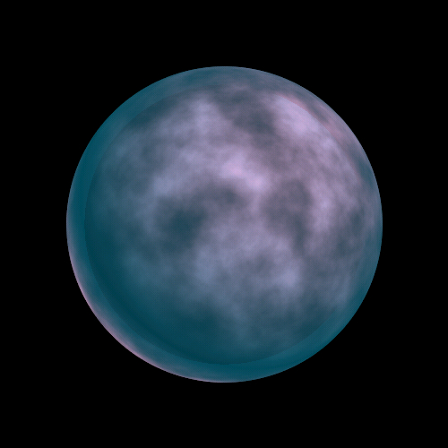
The picture on the left looks a lot more interesting than the previous picture of a number of reasons. The major reason is that it uses a texture that consists of a fractal sum of noise calls:
noise(p) + ½ noise(2p) + ¼ noise(4p) ...
We continue this sum until the size of the next term would become too small to see (ie: the noise would fluctuate faster than about once every two pixels). This results in a logarithmically greater cost than simple noise, depending on image resolution.
For example, in the image on the left I needed to use 8 evaluations in the sum, since any detail smaller than (0.5)8 of the image width would just have contributed random noise to the texture at this resolution.
In the example on the left, a simulation of cloud cover over a watery planet, I used this expression to modulate between the white cloud cover and the dark green-blue planet.
The appearance of a thick transparent atmosphere layer is just a trick — I lighten the planet color beyond a certain radius in the image. Then I apply the cloud texture over this, which creates an illusion that this color modulation is in 3D. The planet then appears to be transparent, with a smaller sphere floating within.
Slide 22 | sum 1/f( |noise| )
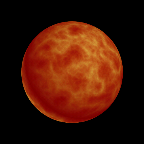
Here instead of a fractal sum of noise, I use a fractal sum of the absolute value of noise:
|noise(p)| + ½ |noise(2p)| + ¼ |noise(4p)| ...
The application of the absolute value causes a bounce or crease in the noise function in all the places where its value crosses zero. When these modified noise functions are then summed over many scales, the result is visual cusps — discontinuities in gradient — at all scales and in all directions. The visual appearance is consistent with a licking flame-like effect, if it's colored properly. In 1984 I started calling this formulation turbulence, since it gives an appearance of turbulent flow.
Slide 23 | sin(x + sum 1/f( |noise| ))
That licking flame effect, with cusps at all scales, pretty well describes the visual appearance of all sorts of turbulent flow. The image to the left was created by taking the turbulence texture from the previous example, and then using it, not to modify color, but to do a phase shift in a simple stripe pattern. The stripe pattern itself is created with a sine function of the x coordinate of surface location:
sin( x + |noise(p)| + ½ |noise(2p)| + ...)
Perturbing the phase of its domain produces a ripple-distortion, similar to the spatial distortion you see when you look through shower glass. On top of this you can also add an inner luminance, as I did back in 1984 with the marble vase shown on the first slide of this talk, to simulate the lovely opalescent translucency found in some kinds of marble.
Slide 24 | Using 3D noise to animate 2D turbulent flow
Next I'm going to show some examples of how to animate flowing textures using noise. The important point to come away with here is that:
You need to use 3D noise in order to do convincing time-varying flow of 2D surfaces.
That extra dimension is needed because turbulent flow has a beautiful randomly coherent appearance that is best handled by treating time as another spatial (and therefore texturable) dimension.
Slide 25 | Flame: noise scales in x,y, translates in z
The corona on the left was made as follows:
- Create a smooth gradient function the drops off radially from bright yellow to dark red.
- Phase shift this function by adding a turbulence texture to its domain.
- Place a black cutout disk over the image.
This creates a fine static image, but how do we animate it? If you just scale the domain of the noise to make the texture flow outward, you get a very fake sort of effect, sort of like those old lightbulb and rotating aluminum foil fireplaces: the texture features move straight outward with no random movement.
To improve this, we use 3D noise. We indeed scale the noise over time, but also, as the animation proceeds, we translate the domain of the noise in its z dimension, out of the image plane. This creates a controlled random flicker in the texture, which complements the outward flow produced by the scaling, and results in remarkably real looking flame animation.
Slide 26 | Clouds: noise translates in x and z
Here we apply the same technique to animating clouds. In this case we use the turbulence texture to phase shift the domain of the flow in y (vertically) rather than radially:
colorMap(y + F(x,y,z))
If you click below to see the animations, you'll see that the animated clouds (as well as the animated flame you saw before) form a cycle. This was done by replacing the perturbation function F(x,y,z) with:
F<sub>2</sub>(x,y,z) = (1–z)*F(x,y,z) + z*F(x,y,z–1)
Notice that F2(x,y,0) = F2(x,y,1). Now we can compute the cloud animation from z=0 to z=1:
colorMap(y + F<sub>2</sub>(x,y,z))
Remarkably, all of the detail in the previous cloud imagery comes from its texture. Here is what the image looks like without the cloud perturbation: a simple vertical color grad.

\/\/\/\/ Missing technology \/\/\/\/
Here were some burned slides describing an ancient java technology and electronic computational machines. There was an information about building a specified FPGA that would render such noises in smoothly 30 fps
/\/\/\/\ Missing technology /\/\/\/\
Slide 27 | Coming next: simplex noise
I'm also developing a different approach to noise, in which the cubic lattice is replaced by a simplicial lattice. This becomes a big win in higher dimensions, starting at noise over R4, and then just keeps getting better. If you evaluate a point based on the influence of vertices of a surrounding simplex, then you only need to do n+1 operations, one per vertex. In contrast, the grid method gets twice as slow with each added dimension, which becomes untenable beyond four dimensions.
Since at each vertex of the simplex you need to do a dot product between items of length n, the total cost of the simplex algorithm is O(n2) with respect to dimension. In contrast, the traditional noise implementation is at least O(2n).
This allows you to do things like procedurally textured BRDFs, which are four dimensional, and become five dimensional when you vary them through time. My current plan is to explain the simplex approach in detail in a paper to be submitted for SIGGRAPH 2001.